Singular Value Decomposition from scratch

PCA’s objective corresponds with SVD

Given any matrix $X$, it is factorized into $U \Sigma V^T $

$X = U \Sigma V^T$

SVD answers 2 important questions asked by PCA:

If we have to cut 1 axis, which one should we cut that minimize the lost of information? Alternatively, what transformation matrix or new coordiante system best approximates the data? (change of basis)
After finding the new coordinate system, what is the distance bewteen all data points?

Traditionally there are 2 steps in computing SVD. The most interesting part is, computing these 2 steps geometrically answer the above 2 questions:

$\begin{align} X^T X &= V \Sigma^2 V^T \\ XV &= U\Sigma \end{align}$

Lets see why!

For consistency of notation, $V$ is change of basis matrix, $U$ is the data distance on new coordinate system and $\Sigma$ scale the data distance with variance in new coordinate system axis.

There is a good SVD visualization. (Basically you could drag the coordinate system around to see which angle has the most variance)

1st question: Which axis should we cut: change of basis matrix

How does computing covariance matrix in 1st step tells us which axis to cut?

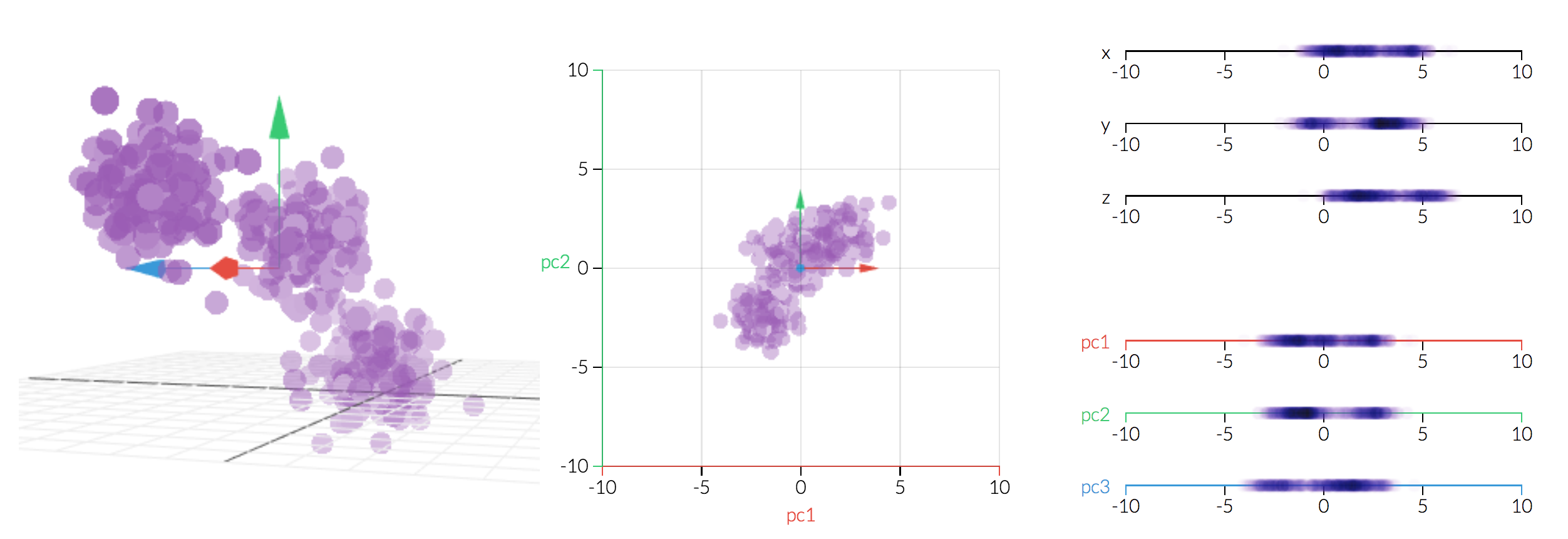
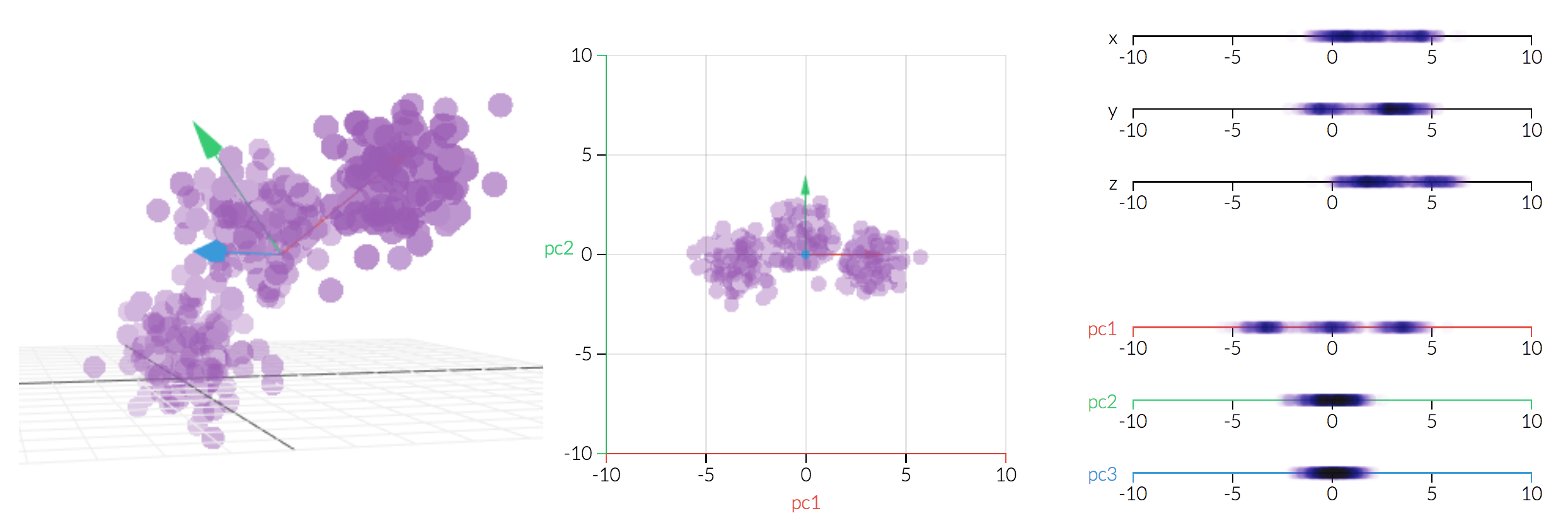
Before change of basis, assuming blue arrow is x-axis, red y-axis, green z-axis.

After change of basis

But if we change the basis by rotating the coordinate system, blue arrow arguably should be the one that gets cut as it has the least variance within the new coordinate system. (notice blue will no longer represents the original x-axis)

Example code:

Lets use the real data to solidify our understanding of change of basis!

Here is some fake data from that approximates SVD visualization graph’s dataset. It is clear that there is a almost upward trend of the data. Assuming matrix $ X $ represents the dataset where rows denotes sample index and columns denotes attributes of each sample.

import numpy as np
from numpy.linalg import svd

X =  np.array([
	[1,1,0.5],
	[2,2,1],
	[3,3,1.5],
	[4,4,2],
	[5,5,2.5],
	[6,6,3],
	[7,7,3.5],
	[8,8,4]
])

U, Sigma, V_transpose = svd(X, full_matrices=False)
Covariance_matrix = np.dot(dataset.T, dataset)
print(Covariance_matrix, U,singularValues,V_transpose)

output:

## Covariance matrix between attributes, x, y, z
[[ 204.  204.  102.]
 [ 204.  204.  102.]
 [ 102.  102.   51.]]

## U, reduced, not full-rank(full rank just pad number to artificially creates orthornormal square matrix)
[[-0.070014   -0.97259152  0.02717264]
 [-0.14002801  0.04421983  0.98874033]
 [-0.21004201 -0.01941955 -0.02452013]
 [-0.28005602  0.08843966 -0.05259622]
 [-0.35007002  0.02480028 -0.05081823]
 [-0.42008403 -0.0388391  -0.04904025]
 [-0.49009803 -0.10247848 -0.04726227]
 [-0.56011203  0.17687931 -0.10519243]]

## Sigma
[  2.14242853e+01   1.93007163e-15   2.53327545e-31]

## V_tranpose, othornormal 
[[-0.66666667 -0.66666667 -0.33333333]
 [ 0.74535599 -0.59628479 -0.2981424 ]
 [-0.          0.4472136  -0.89442719]]

[-0.66666667 -0.66666667 -0.33333333] is the new angle (column vector) that results in most variance. Notice that (x,y) co-varies 2 times than (y,z) or (x,z) in covariance matrix, which coincides with the 1st new angle in SVD.

$X^T X$ could be thought as computing covariance matrix between attributes. Each entry in covariance matrix represents attributes similarity between 2 attributes.)

$\begin{align} X &= U \Sigma V^T \\ X^T X &= {(U\Sigma V^T)}^T (U \Sigma V^T) \\ X^T X &= {(V\Sigma U^T)} (U \Sigma V^T)\\ X^T X &= V {\Sigma}^2 V^T \end{align}$

where $V {\Sigma}^2 V^T $ is the diagonalization of $X^T X$

It might not seem straightly obvious as why we compute covariance matrix other than mathematically it cancels out U.(orthonormal eigenvectors transpose multiplication results in identity matrix) Here are 2 ways to see intuitively why computing covariance matrix (i.e. $ X^T X = V {\Sigma}^2 V^T$) is directly computing the new coordinate system that maximizes variance.

1. solving determinant = 0 to find eigenvalue

$\begin{align} X^T X &= V {\Sigma}^2 V^T \\ X^T X V &= {\Sigma}^2 V \\ (X^T X - {\Sigma}^2 I) V &= 0\\ \det(X^T X- \Sigma^2 I) &= 0 \end{align}$

Gemetrically, it corresponds to rotate, stretches and rotates back and variance is maximized in that new coordinate system.

But why does rotating covariance matrix til linear dependence ( $\det(X^T X- \Sigma^2 I) = 0$ ) implies $ \DeclareMathOperator*{\argmax}{arg\,max} \argmax $ variance in rotating tranformation matrix ($XV = U\Sigma$)? (try to picture 2 rotations simultaneously side by side)

Focusing on $\det(X^T X- \Sigma^2 I) = 0$, rotating the covariance matrix (notice not data matrix) is maximizing the variance (i.e. $\Sigma$) in new coordinate system under constraint. The contraint is linear dependence. Each column vector in covaraicne matrix could only move along in 1 axis (recall $\det(X^T X- \Sigma^2 I) = 0$) until rotation squishes eigenvector $V$to 0.

$\Sigma^2$ is only maximized if there is a real solution of eigenvector.

A good visualizationof such constraint in rotating covaraince matrix is here:

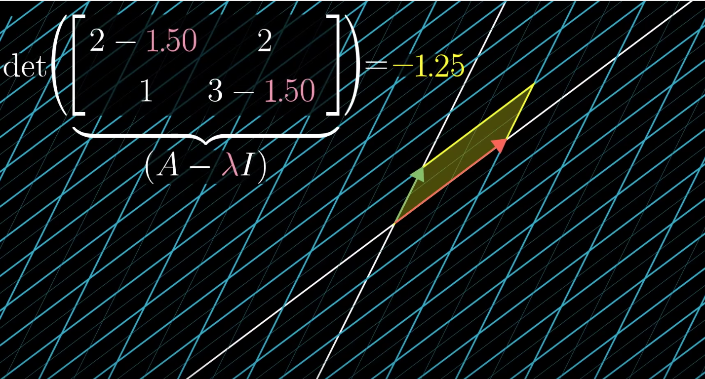
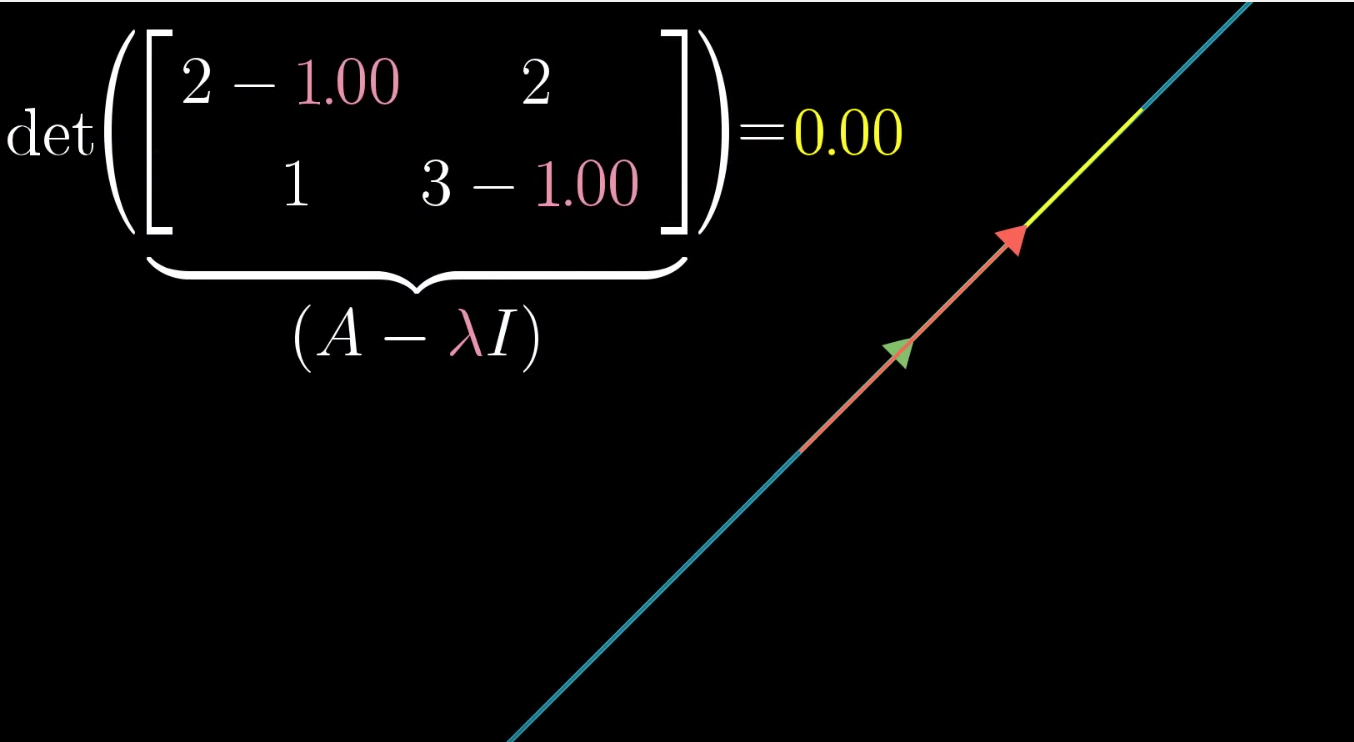
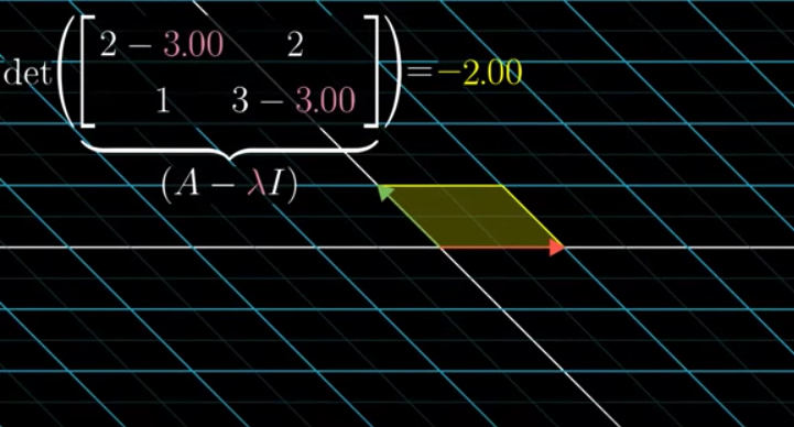
(note: this above example is not a symmetric matrix like covariance matrix)

2. Solve for eigenvector instead! The direction that maximizes variance is already implied in the covariance matrix

Personally I find this explanation more intuitive. If you understand how to computing pagerank, this should be rather straightforward. Here is a very good water reserviors and pumps analogy to visualize pagerank in terms of matrix multiplication.

Covaraince matrix is a symmetric matrix that could be viewed as:

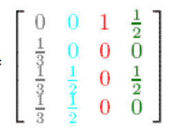
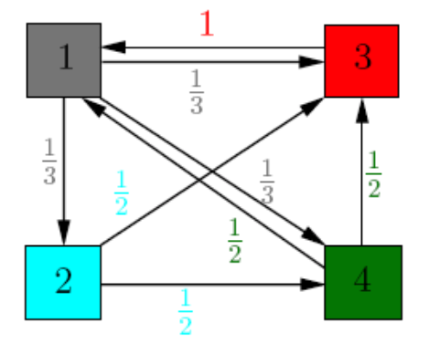
where each node represents an attribute (i.e. x,y,z) and each edge denotes a covariance entry between 2 attributes.

Recall:

$X^T X V = {\Sigma}^2 V$

Solving $V$ is essentially solving how much weights should be given to each attributes given the dynamic system of interaction between attributes as denoted in covariance matrix. The resulting weights vector is eigenvector for change of basis.

To compute with power iteration until it converges, start with random vector $v$:

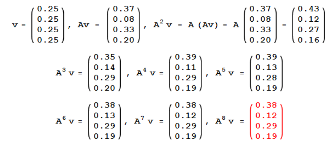
Iterating $v, Av, …, A^k v$ converges to equilibrium value of weights vector.

For a random surfer perspective, we can model the process as a random walk on graphs with edges as probability ended up on outgoing node. $v, Av, …, A^k v$ converges to final probabilitic vector.

Both weights vector or probabilistic vector denotes eigenvector. It concludes how important that attribute is and hence how much to rotate in stationary distribution.

Switching from probabilitic or dynamic system point of view to just linear algebra, this eigenvector could be directly computed by solving $V$ in $X^T X V = {\Sigma}^2 V$:

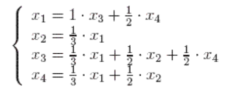
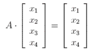
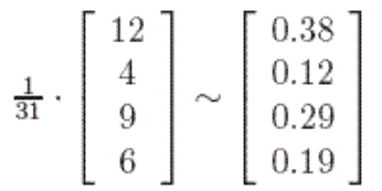
Geometrically, eigenvectors are vectors that did no change after transformation matrix. This happens to coincides with page rank’s “stable fraction”.

$\begin{align} Ax &= \lambda x \\ Px &= x \end{align}$

Eigenvector intuitively could be seen as “stable fraction” vector. And this stable fraction vector indicates the new coordinate system.

After computing the new change of basis matrix, we could answer the 2nd question.

2nd question: given new change of basis, how to compute distance of each data point on the new coordinate system?

Recall there are 2 steps in computing SVD:

solve $X^T X = V\Sigma^2 V^T$
solve $XV = U\Sigma$

1st step already does most of the heavy lifting. 2nd step is rather strightforward: solve $U$ with $V$ and $\Sigma $ from step 1. The interesting part of 2nd step is geometrically computing $XV$ is actually computing the distance between the new coordinate system and data points. To see this, we need to look at projection of $X$ onto subspace $V$ by taking dot products $XV$.

Here is a visual picture of computing distance between data points and new axis:

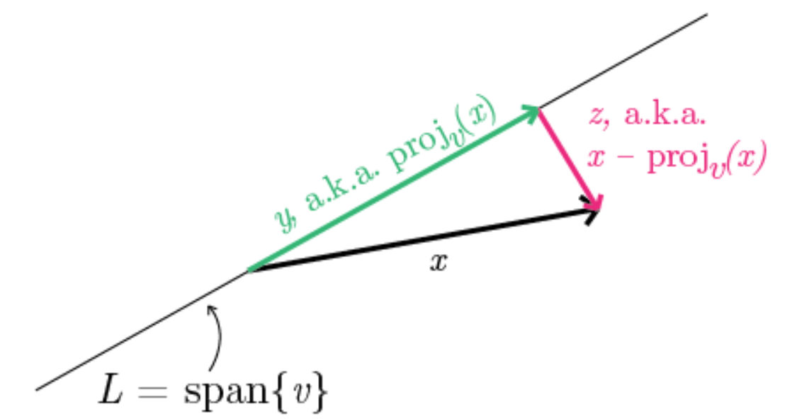
$ proj_v(x)$ linear maps input vector $x$ and output projection of $x$ onto $v$ where $ proj_v(x): \mathbb{R^n} \to \mathbb{R^n} $

squared length of projections is computed by taking dot product: $ |x \cdot y| $

$ proj_v(x)$: v scaled by inner product of x and v.

$XV$ is projection length of all data points $x_i$ onto 3 new coordinate lines spanned by $V$. Each entry is dot products $ x_i \cdot v_i $. The squared norm of $ XV $ denotes sum of squared lengths of projections of data onto line spanned by $v$

$\begin{align} proj_v(x) &= (x\cdot v) \cdot v \\ \sum_{i} {x_i}^2 &= (proj_v(x))^2 + (dist_v(x))^2 \\ \sum_{i} {x_i}^2 - (dist_v(x))^2 &= (proj_v(x))^2 \\ (dist_v(x))^2 &= (\sum_{i=1}^{n} {x_i}^2) - |x \cdot v| \end{align}$

$dist_v(x)$ distance of $x $ from line spanned by unit vector $v$. Given x is constant, maximizing sum of squared lengths of projections is the same as minimizing squared Euclidean distance between projected line and data points

Formally:

$\DeclareMathOperator*{\argmax}{arg\,max} \argmax_{||v||=1} \frac{1}{m} \displaystyle \sum_{i=1}^{m} {\langle x_i, v \rangle}^2$ $\DeclareMathOperator*{\argmax}{arg\,max} \argmax_{v:||v||=1} |Xv|$ $\DeclareMathOperator*{\argmax}{arg\,max} v_2 = \argmax_{v \bot v_1, ||v|| =1} |Xv|$

SVD from scratch with power iteration

import numpy as np
from numpy.linalg import norm
from random import normalvariate
from math import sqrt
 
def random_unit_vector(size):
    unnormalized = [normalvariate(0, 1) for _ in range(size)]
    norm = sqrt(sum(v * v for v in unnormalized))
    return [v / norm for v in unnormalized]
 
def power_iterate(X, epsilon=1e-10):    
    """ Recursively compute X^T X dot v to compute weights vector/eignevector """
 
    n, m = X.shape
    start_v = random_unit_vector(m) # start of random surf
    prev_eigenvector = None
    curr_eigenvector = start_v
    covariance_matrix = np.dot(X.T, X)
 
    ## power iterationn until converges
    it = 0        
    while True:
        it += 1
        prev_eigenvector = curr_eigenvector
        curr_eigenvector = np.dot(covariance_matrix, prev_eigenvector)
        curr_eigenvector = curr_eigenvector / norm(curr_eigenvector)
 
        if abs(np.dot(curr_eigenvector, prev_eigenvector)) > 1 - epsilon:            
            return curr_eigenvector

def svd(X, epsilon=1e-10):
    """after computed change of basis matrix from power iteration, compute distance"""
    n, m = X.shape
    change_of_basis = []
 
    for i in range(m):
        data_matrix = X.copy()
 
        for sigma, u, v in change_of_basis[:i]:
            data_matrix -= sigma * np.outer(u, v) 
 
        v = power_iterate(data_matrix, epsilon=epsilon) ## eigenvector 
        u_sigma = np.dot(X, v) ## 2nd step: XV = U Sigma 
        sigma = norm(u_sigma)  
        u = u_sigma / sigma
 
        change_of_basis.append((sigma, u, v))
     
    sigmas, us, v_transposes = [np.array(x) for x in zip(*change_of_basis)]
 
    return sigmas, us.T, v_transposes            

if __name__ == "__main__":    
    dataset = np.random.random_sample((8, 3))
    results = svd(dataset)
    print("sigmas", results[0])
    print("u: data points in new coordinate system", results[1])
    print("v transpose: change of basis matrix", results[2]) 

Reference and credits:

here

(All credit goes to these brilliant sources, I merely put together highlights for intuitions.)

Appendix:

If you prefer change of basis or transformation matrix at the front and magnitude vector at the end, you could think as:

$U\Sigma V^T = {V^T \Sigma U}^T$

this just requires you to transpose the dataset matrix first.