Introduction of Linear Programming(LP) and convex optimization. Reframing linear regression, support vector machine as convex optimization.

Optimization is slightly difficult to wrap our head around when first time hear about. Linear Programming is a good introduction to the idea of optimization.

Linear Programming using simplex method and its graphical meaning

First we run an entire simplex computation:

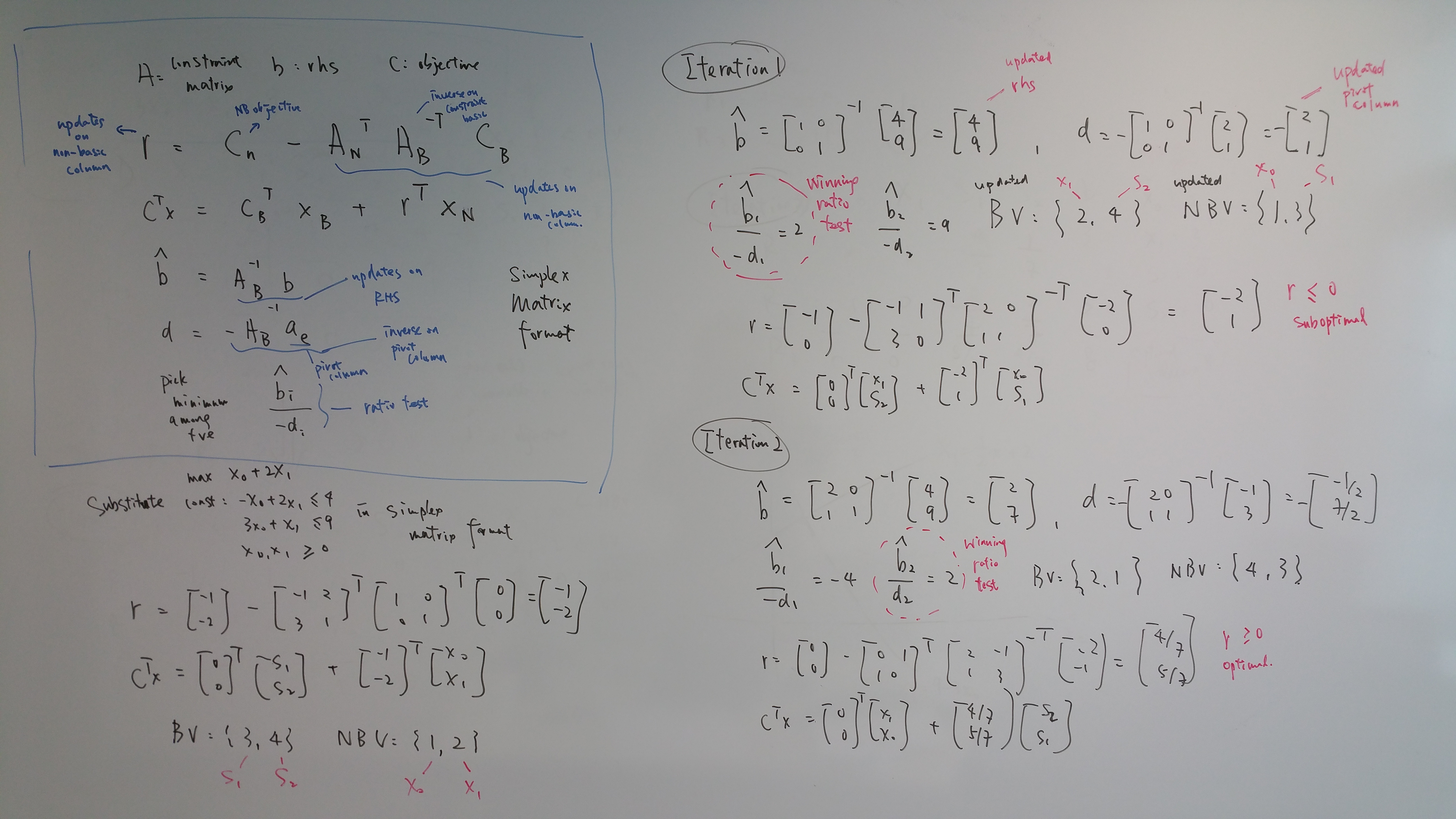
Pivoting: determine entering & leaving variables and using ratio test to determine pivot row

Basic feasible solution: given n variables and m constraints (n>m), basic feasible solution (BFS) is obtained by setting n-m variables non-basic variables (NBV) to 0 to solve for m variables Basic Variables (BV) i.e. just pick 1 variable and set rest to 0 in each constraint. If LP has optimal solution, there could be a set of points and at least 1 of these set of points is extreme point

Pivoting is trying out extreme point according to objective function and adjacent basic fesible solution by changing 1 variable at 1 time. We pick pivot point (extreme point) by picking pivot row and pivot column(entering variable). Entering variable is decision variables that causes the biggest increase in objective function. Variables that are not entering variable are slack variable which turns inequality into equality. Existence of slack variable indicates room from constraint, allow such extreme point not on the constraint line.

Then use elimination row operation (ERO) to find adjacent BFS (adjacent extreme point). Intuitively, ERO is looking for extreme points in constraints.

Then we get difference between 2 constraints changing 1 variable in BFS to adjacent BFS, given we have the same variable in BFS (i.e. when constraints meet how much difference in that variable in adjacent BFS). Our goal is to convert to identity [1 0 1 0] that measure difference.

Then we apply ratio test to decide pivot row. Intuitively ratio test determines largest value entering variable (x or y) could be without violating constraints. i.e. amount all constraints the smallest so it wont violate other constraints when we zero out all other decision variables.

Then we recursively apply ERO and updates objective until there is no negative left.

Graphically:

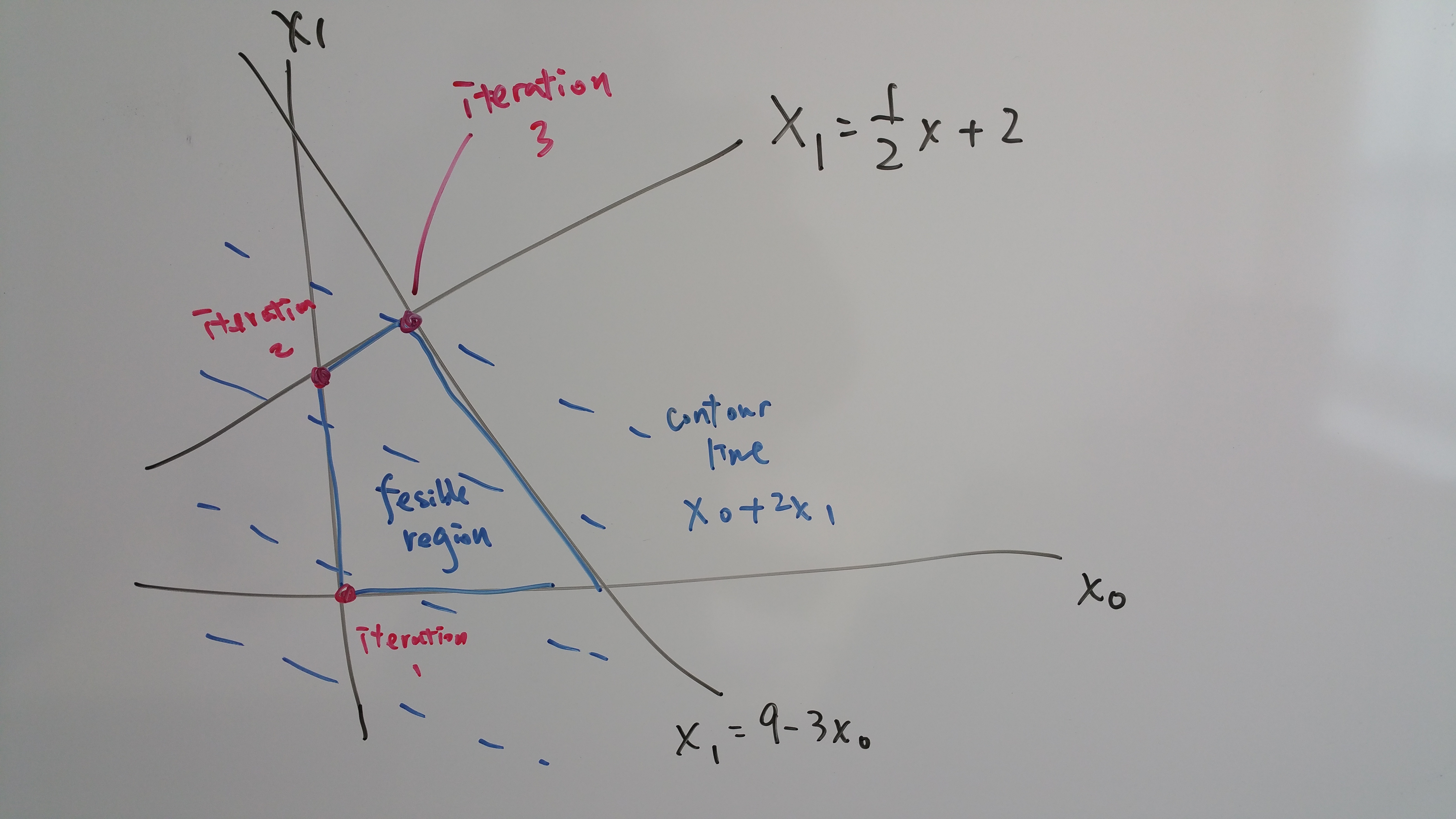
The more important part is visualizing LP in the above graph. When minus contraint with objective function, you are left with SLOPE DIFFERENCE. Slope difference is the shared area between objective line and constraint line difference i.e. potential for constraint line to go further for a higher value. In constrast, when minus 1 constraint from another, we looking for point that coincides, then see how that slope difference translate to value at that point.

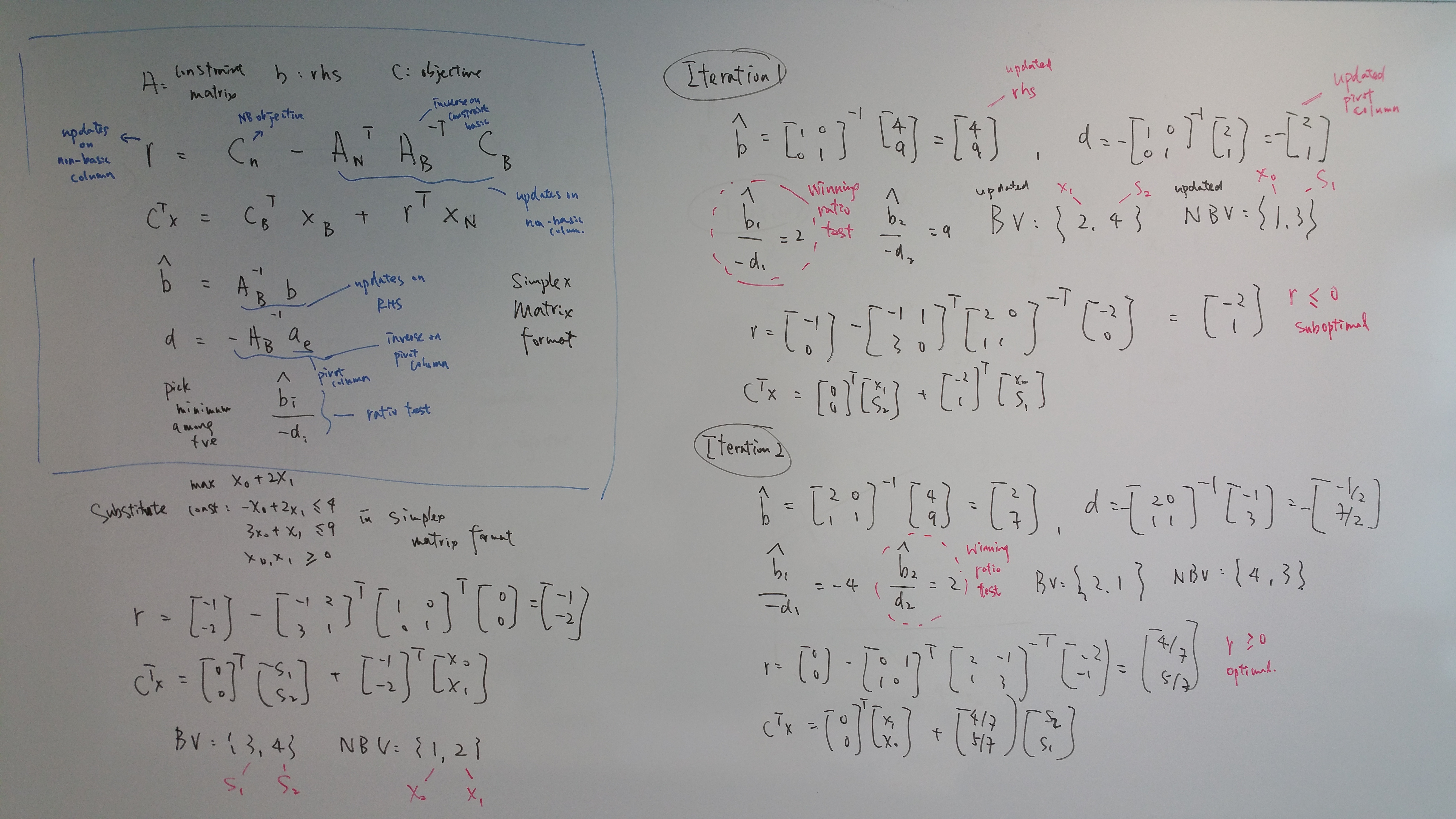
Formally, simplex in matrix form:

I wrote some python code to demonstrate simplex solver from scratch.

"""
Author: Steven Wong
This software has not been tested rigoriously and not meant to be distributed commercially.
"""

import numpy as np
from operator import sub

class LinearProgram(object):
	"""LinearProgram"""
	def __init__(self, A, b, c):		
		self.constraints = A
		self.rhs = b
		self.obj = c	
		self.updated_obj = [ -x for x in self.obj] 
		self.BV = []
		self.NBV = []

		self.canonical_simplex_tableau()
		
		
	def get(self, mat, col_list):
		"""get A_bv, A_nbv, c_bv, c_nbv i.e. constraints matrix n objective vector with only BV or NBV columns"""
		np_mat = np.matrix(mat)
		# print(b[:,col_list])
		return np_mat[:,col_list]

	def canonical_simplex_tableau(self):
		"""add slack variables + init BV, NBV"""

		self.num_constraints = len(self.constraints)
		num_decision_variables = len(self.constraints[0])
		self.NBV = [i for i in range(num_decision_variables)]

		zeros = [0] * self.num_constraints
		self.updated_obj += zeros
		augmented_matrix = [r + zeros for r in A]			
		col = 1
		for row, _ in reversed(list(enumerate(augmented_matrix))):			
		 	# print(augmented_matrix[row][-col])
		 	augmented_matrix[row][-col] +=1
		 	col += 1	
		 	self.BV.append(len(augmented_matrix[0])-row-1) ## init BV
		self.augmented_matrix = augmented_matrix	

					
	def simplex_solve(self):
		""" keep looping if still negative in objective functoin"""
		optimal = 1
		loop = 1
		while(optimal):
			print("\n")
			print("ITERATION:", loop)
			loop +=1
			self.entering_variable()
			self.update_obj()

			for i in range(len(self.constraints)):
				if self.updated_obj[i] < 0:
					break
				optimal = 0		
		self.calculate_optimal()
		print("\n")
		print("SOLUTION: ", self.b_hat, self.opt)

	def calculate_optimal(self):
		self.obj += [0] * len(self.constraints)
		self.A_bv = self.get(self.augmented_matrix, self.BV)
		self.b_hat = np.dot(self.A_bv.I, self.rhs).tolist()[0]
		self.x = [0] * len(self.augmented_matrix[0])
		for i, j in zip(self.BV, self.b_hat):
			self.x[i] = j
		
		self.x = np.matrix(self.x)
		self.obj = np.matrix(self.obj)
		self.opt = self.obj.dot(self.x.T)


	def update_obj(self):
		""" 
		r = C_n - A_n.T * A_b.-T * C_b
		find linear combination that turn BV into identity
		
		+ use that linear combination to update NBV objective value
		
		+ turn all C_bv into zeros"""
		
		print("C_nbv: ", self.get(self.updated_obj, self.NBV))
		print("C_bv: ", self.get(self.updated_obj, self.BV))
		print("A_bv inver, trans: ", self.get(self.augmented_matrix, self.BV).I.T)
		print("A_nbv trans: ", self.get(self.augmented_matrix, self.NBV).T)

		A_nbv_T = self.get(self.augmented_matrix, self.NBV).T
		A_bv_I_T = self.get(self.augmented_matrix, self.BV).I.T
		c_nbv = self.get(self.updated_obj, self.NBV)
		c_bv = self.get(self.updated_obj, self.BV).T

		temp = A_nbv_T.dot(A_bv_I_T).dot(c_bv)
		print(temp, c_nbv)
		# c_nbv = map(sub, c_nbv.tolist(), temp.tolist())
		c_nbv = [a - b for a, b in zip(c_nbv, temp.T)][0].tolist()[0]
		# c_nbv = c_nbv.tolist() - temp.tolist()

		print("c_nbv",c_nbv)
		
		self.updated_obj = [0] * len(self.augmented_matrix[0])		

		for i, j in zip(self.NBV, c_nbv):
			self.updated_obj[i] = j
		print("objective row", self.updated_obj)

		# self.get(self.obj, BV).zeros() # zero out c_bv


	def entering_variable(self):
		""" 
		Pivoting 
		1. pivot col/entering variable 
		2. ratio test to pivot row
		3. update NBV n BV 
		"""

		min_value = min(self.updated_obj)
		# max_index = [i for i, j in enumerate(self.obj) if j == max_value]
		self.pivot_col_index = self.updated_obj.index(min_value) 
		
		self.A_bv = self.get(self.augmented_matrix, self.BV) # constraints with only BV as column
		print("A_bv:", self.A_bv)
		self.b_hat = np.dot(self.A_bv.I, self.rhs)
		print("b_hat: ",self.b_hat)

		self.pivot_col = self.get(self.augmented_matrix, self.pivot_col_index)		
		self.d = np.dot((-self.A_bv.I), self.pivot_col)		
		self.ratio_test = (-self.b_hat/self.d.T).tolist()[0] # convert np back to array		
		
		# self.pivot_row_index = self.ratio_test.index(min(self.ratio_test))		
		self.pivot_row_index = self.ratio_test.index(min(i for i in self.ratio_test if i > 0))		
		print("BV, NBV before", self.BV, self.NBV)

		## update BV
		self.BV[self.pivot_row_index] =\
			self.pivot_col_index		
		## update NBV
		compare = [i for i in range(len(self.augmented_matrix[0]))]		
		self.NBV = list(set(self.BV)^set(compare))
		print("updated BV, NBV: ", self.BV, self.NBV)


if __name__ == "__main__":


	# constraint matrix
	A = [[-1,2],
	     [3,1]]	     
	# rhs
	b = [4,9]	
	# objective function
	c = [1,2]


	LP = LinearProgram(A, b, c)
	LP.simplex_solve()

Linear Regression as convex optimization

Optimization with projection matrix (more commonly known as “fitting the best line” by setting partial derivatives to 0)

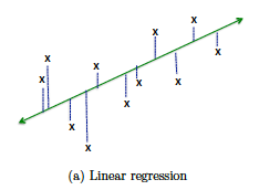
Least squares projection approximation, also known as linear regression, is clearest application of convex optimization. In linear regression, Ax = b has no solution because of more equations than unknowns. The matix has more rows than columns. We could compute such optimization from both linear algebra and calculas perspective.

Projection matrix to optimize for the best fit line

By projecting $b$ on to column space we are solving the same problem as fitting the best line. Squared length of $ \left\Vert Ax - b \right\Vert^2 $ is minimized. To see this:

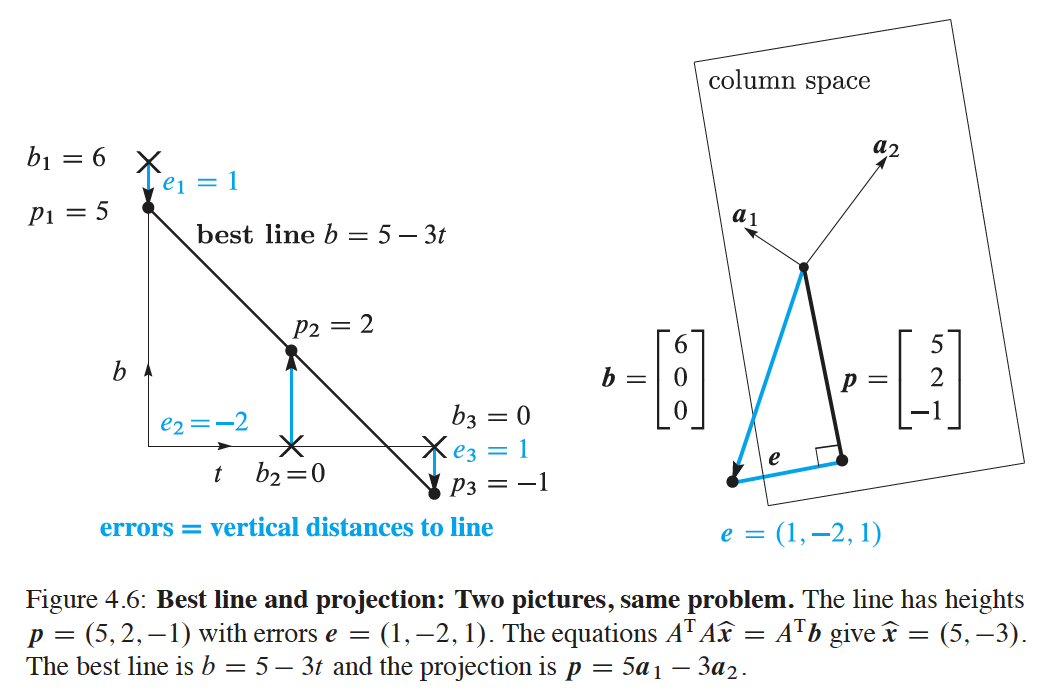
Note: (on the right) is minimizing $e$ perpendicular distance to column space whereas (on the left) is minimizing vertical distance geometrically

Proof of projection matrix:

$\begin{align} Ax &= b \quad \text{where b = p + e, is not solvable}\\ A \hat x &= p \quad \text{is solvable} \hat x \text{means combination in A column space} \\ A^T(b-A \hat x) &= 0 \quad \text{since e in nullspace and } \perp \text{to A's column space } \\ A^T A \hat x &= A^T b \\ A \hat x &= A (A^T A)^{-1} A^T b \quad \text{where } A (A^T A)^{-1} A^T \text{ is the projection matrix of b on A}\\ \end{align}$

Instead of solving $Ax = b $, we assume $b = p$ and solve for $A \hat x = p $ where $p$ represents projection on column space of A and also the “best fit line”. This reconciles 2 seemingly differnt objectives (vertical vs orthogonal) in 2 graphs above as the same.

A comparison of squared length distance for best line(on the left) vs direct projection line on column space(on the right):

$\begin{align} || Ax - b ||^2 &= || Ax-p ||^2 + || e ||^2 \quad \text {Pythagorean Theorem} \\ \end{align}$

for right hand of above equation:

$\bullet $ $x$ is arbtrary straight lines on left graph, combination on right graph

$\bullet $ $Ax$ is arbitrary vectors on column space

$\bullet $ $p $ is b’s projected part on column space

$\bullet $ $e $ is perpenducular part in left null space

$\bullet $ $Ax - p $ is misses from direct projection measured on column space

Picking any non best lines on the left graph translates to positive $ \left\Vert Ax - p \right\Vert^2 $ distance on the right graph (i.e. non zero vector adding to $p$). $ \left\Vert Ax - b \right\Vert^2 $ is minimized when $ \left\Vert Ax - p \right\Vert^2 $ is zero where $ Ax = A\hat x = p$. Projection matrix formula $A^T A \hat x = A^T b$ find the right combination $\hat x$ to project $b$ onto $A$. Direct projection on right graph happens to coincide with finding best fit line on left graph.

Below is 4 fundamental subspace analysis:

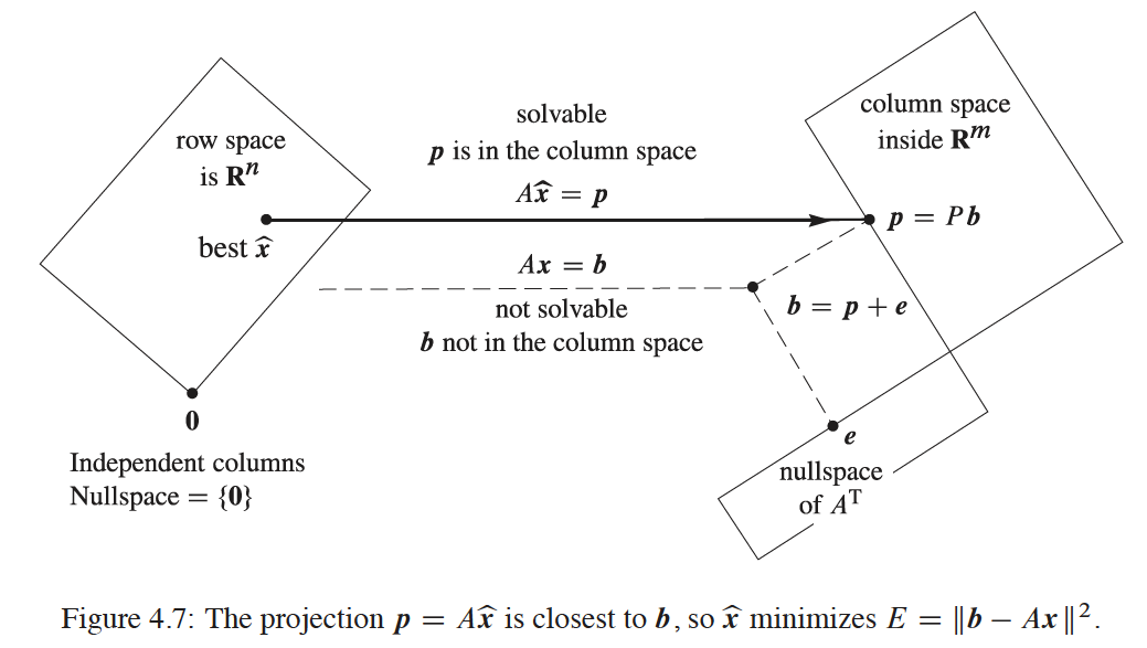
calculas perspective: => calculas set to 0 is same as projection matrix proof: => only show example partial derivative calculation to show its also projection matrix => convex graph

Alternatively from calculas, by taking partial derivative of error function and setting it to zero results in same equation $ A^T A \hat x = A^T b $. To see why:

$\begin{align} e_i &= b_i - C - Dt_i \quad \text{where C D is } \hat x \\ \left\Vert Ax - b \right\Vert^2 &= (C + Dt_1 - b_1)^2 + \cdots + (C + Dt_m - b_m)^2 \quad \text{summing up all errors} \\ \end{align}$

To compute the minimum of convex function, calculas sets partial derivatives $ \frac{\partial E}{\partial C} $ and $ \frac{\partial E}{\partial D} $ to zero and resulted in following equation to solve.

$\begin{bmatrix} m & \sum t_i \\ \sum t_i & \sum t_i^2 \end{bmatrix} \begin{bmatrix} C \\ D \end{bmatrix} = \begin{bmatrix} \sum b_i \\ \sum t_i b_i \end{bmatrix}$

Look closely this is the same equation as $ A^T A \hat x = A^T b $!

$A^T A = \begin{bmatrix} 1 & \cdots & 1\\ t_i & \cdots & t_m \end{bmatrix} \begin{bmatrix} 1 & t_1 \\ \vdots & \vdots \\ 1 & t_m \end{bmatrix} = \begin{bmatrix} m & \sum t_i \\ \sum t_i & \sum t_i^2 \end{bmatrix}$ $A^T b = \begin{bmatrix} 1 & \cdots & 1\\ t_i & \cdots & t_m \end{bmatrix} \begin{bmatrix} b_i \\ \vdots \\ b_m \end{bmatrix} = \begin{bmatrix} \sum b_i \\ \sum t_i b_i \end{bmatrix}$

SVM

Since there are quite some very important variables in SVM to keep track off and different textbooks give them different names, it might be easier to understand if defined beforehand.

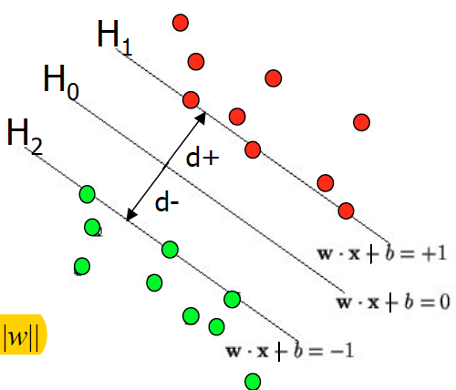
$H_0$ is decision boundary/medium/hyperplane/hypothesis $\vec{w}$ is normal $\vec{w}$ w is called normal and $perp$ to decision boundary $H_0$ we are optimizing for. $H_1$ and $H_2$ are gutters where support vectors, i.e. the closest +ve and -ve data point, lies on Gutters and decision boundary together form a street since it looks like a street.

$b$ is shift/bias/offset that primarily shift the medium line that originally pass through the origin

$x_+$ is datapoints with +ve label, $x_-$ is datapoints with -ve label

Labeled datasets: $$ D = {(x_i, y_i)

i = 1,…,m, x_i \in\mathbb{R}^n, y_i \in {1,-1}}$$

Formulate trainable parameters in cost function to do classification. As a convex optimization task, we want to spread the gutter as far away until it reaches.

$\begin{align} \vec{w} \cdot \vec{x} = 0 \end{align}$

Decision rule or hyperplane is the line that separates which separates all data points with +ve labels from those with -ve labels. i.e. \ (H_0\) Graphically, $\vec{w} \cdot \vec{x} + b = 0$ can be expressed as $y = ax + b$. By setting $\vec{w} \cdot \vec{x} + b$ to zero, we are optimizing for $\vec{w}$ and $b$ that maximizes the margin.

Next step we need to define gutters

$\begin{align} \vec{w} \cdot \vec{x_1} + b &\ge 1 \\ \vec{w} \cdot \vec{x_1} + b &\le -1 \end{align}$

add mathematical convenience variable y, both equation becomes the same as when y = -1 it flips the sign

$\begin{align} y_i (\vec{w} \cdot \vec{x_1}) + b &\ge 1 \\ y_i (\vec{w} \cdot \vec{x_1}) + b &\ge 1 \\ y_i (\vec{w} \cdot \vec{x_1}) + b -1 &\ge 0 \quad \text{for all points}\\ y_i (\vec{w} \cdot \vec{x_1}) + b -1 &= 0 \quad \text{for support vectors that lies on gutter} \end{align}$

We can see inner product between data points and normal determines the sign of data points. Inner product is equivalent to project data onto normal, if the projected length is longer than margin it is a +ve sample, otherwise it is -ve.

here is a good visualization

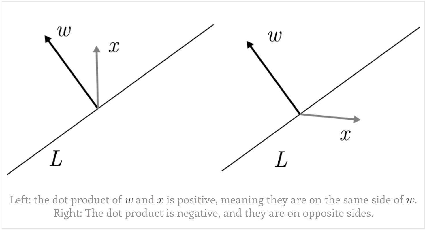
Projection means take only the components of x that point in the direction of w. Another way to think of this is that the projection is x, modified by removing any part of x that is perpendicular to w.

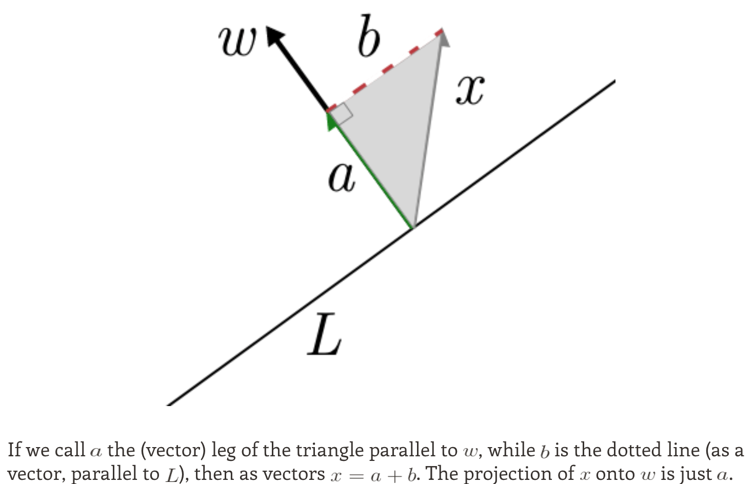
Now finally we are ready to formulate SVM optimization objective. All we need to do is substitute constraints into decision boundary and dot the difference between +ve and -ve support vectors with unit normal vector. Projection onto normal with normal equals to 1 directly calculates the street width.

$\begin{align} y_i (\vec{w} \cdot \vec{x_1}) + b -1 = 0 \quad \text{for support vectors that lies on gutter} y_i (\vec{w} \cdot \vec{x_1}) = 1 - b \end{align}$

As such, final form of optimization function: $\begin{aligned} & \min_{w} \frac{1}{2} \| w \|^2 & \\ \text{subject to \ \ } & (\langle x_i, w \rangle + b) \cdot y_i \geq 1 & \text{ for every } i = 1, \dots, m \end{aligned}$

Intuition of scaling normal

It might not be immediately clear how $\min_{w} \frac{1}{2} | w |^2 $ wiggle gutters and medium to the optimal form.

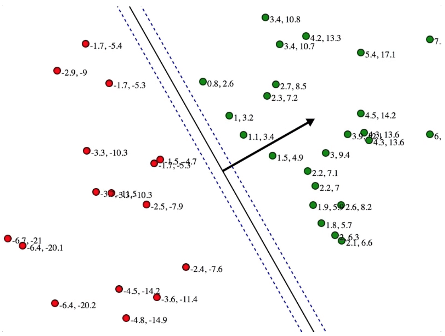
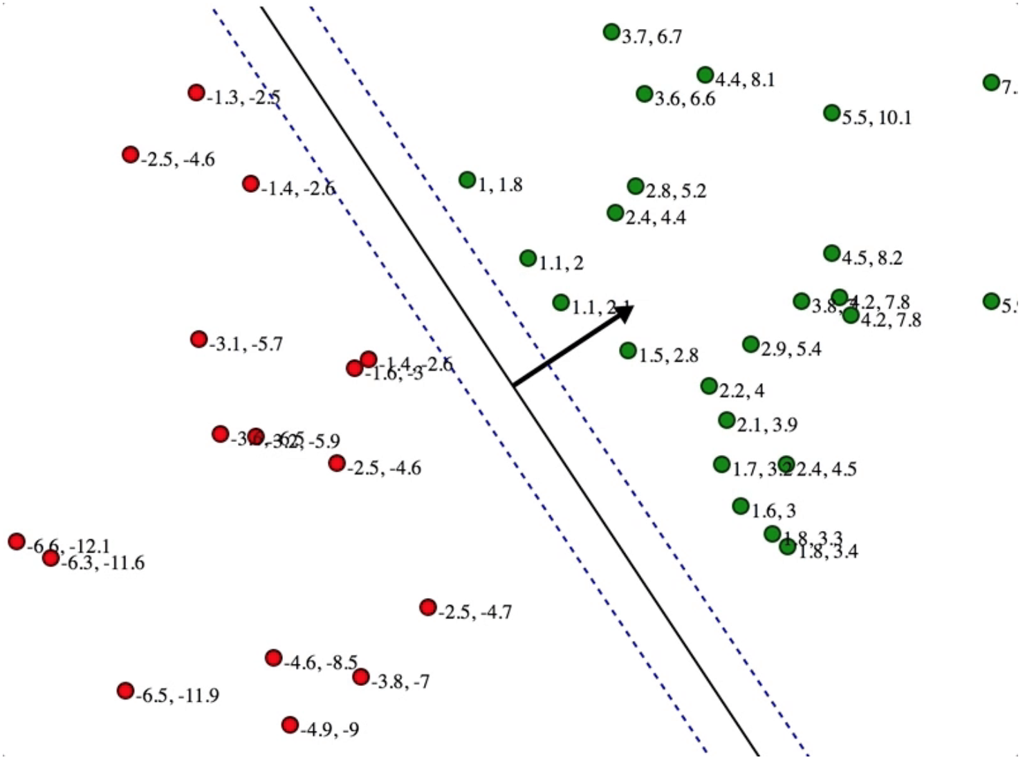
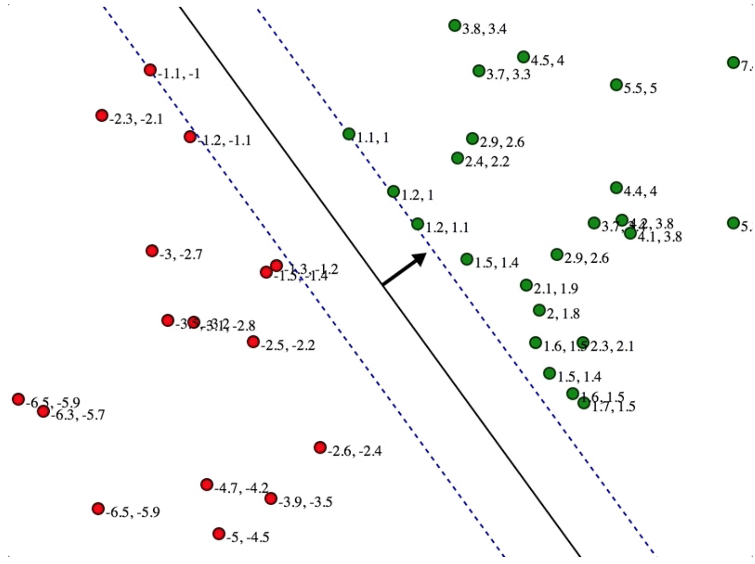
We could see the smaller the normal, the wider the gutter. This corresponds with maximizing street width $\frac{2}{\vec{ |w|}}$.

If we look closely, there is a scaling variable c for support vectors on gutters.

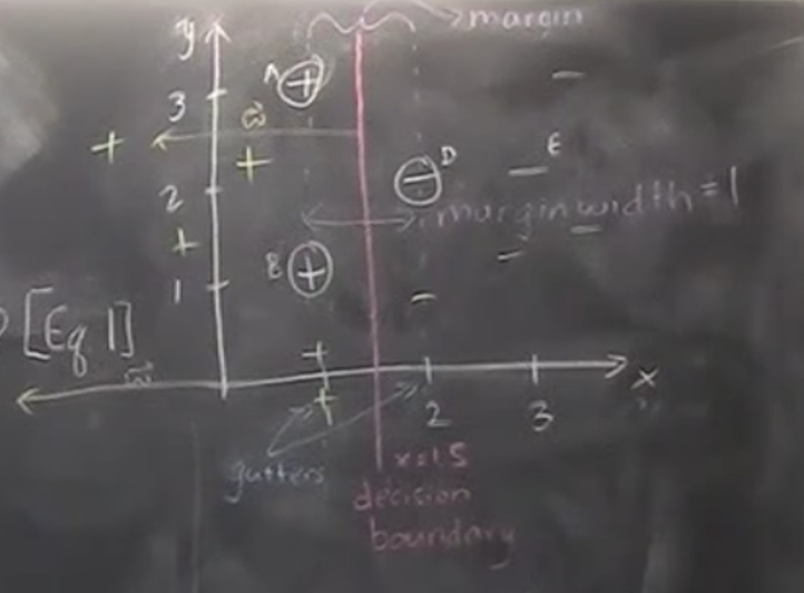
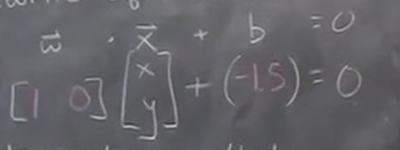
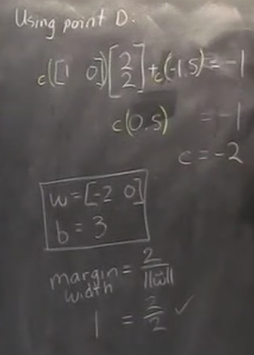
$\begin{aligned} c \cdot \vec{w} \cdot x = 1 \end{aligned}$

We could see the bigger x is, the smaller scaling variable c is going to be, given $\vec{w}$ is unchanged. This exactly explains the above figure when the normal arrow is $c \cdot w$ and the gutter is x.

Since such objective formulation is convex so we could optimize to get global minimal.

reference:

Yong Wang, amazing Professor from SUNY Binghamton

Gilbert Strand, amazing Rhodes Scholar from MIT teaching 18.06

Stephen Boyd: Introduction to convex optimization

MIT SVM for idiots

MIT 6.034 AI Patrick Winston

Jeremy Kun, amazing Google Software Engineer, Mathematics PhD from UI Chicago

Jessica Noss, amazing Google Software Engineer again, MIT AI researcher